
Image Classification of X-Ray scans using Convolutional Neural Networks
Artificial Intelligence is making the lives of doctors, patients and hospital administrators easy by performing the tasks that are typically done by humans with less effort and cost. HealthCare industry will be one of the highest growth industries in the field of AI which is projected to reach $150 billion value by 2026.
The healthcare industry is in a huge transformation where technology is the driving force. In this shift, although AI has done tremendous progress it is not yet sophisticated to perform the final diagnosis; it is simply meant to assist medical professionals who give their final diagnosis.
Today in this blog post we can understand how Image Classification using AI can help doctors/radiologist to decrease their workload and increase their efficiency on another research.
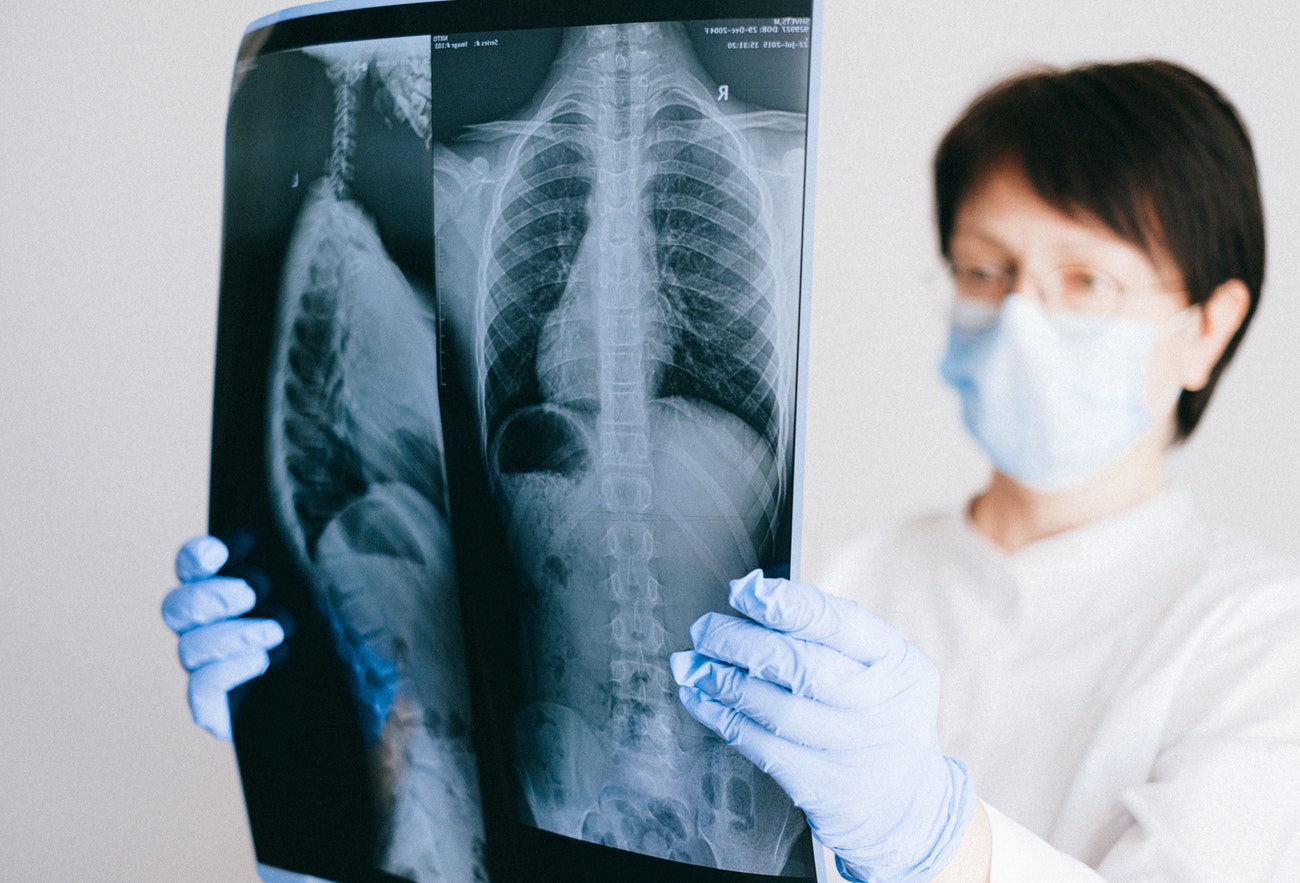
Generally, Tuberculosis can be screened using chest X-Ray scans. It is not possible for a layman to distinguish between the lungs of a normal person and the person having tuberculosis. We need Radiologist/Doctor who will observe the key patterns in the X-rays and identifies if a person has Tuberculosis or not. Radiologist usually gets huge number of X-rays or other type of scans to identify different disease conditions. In order to reduce the workload of Radiologist and to make the process quicker and automated, we can develop a classification models which can give the predictions based on the historical labelled data.
Build you own AI Model
In this blog post We will go through step by step process of building an image classifier to detect if the person has Tuberculosis or not using Chest X-Rays.
Step 1 - Import Libraries to Build Model
#Importing the necessary libraries
import pandas as pd
import numpy as np
import glob
from sklearn.model_selection import train_test_split
from keras.preprocessing import image
import keras
from keras.applications import vgg16
from keras.models import Sequential
from keras.layers import Dense, Dropout, Flatten, Conv2D, MaxPooling2D
from pathlib import Path
import joblib
import warnings
warnings.filterwarnings("ignore")
Step 2 - Get Data
You can get the publicly available from many websites. Here I took the data that is available in Kaggle. Download the data from the above link to your computer or you can place in any cloud service provider storage application. Here I download all the images in to one folder.
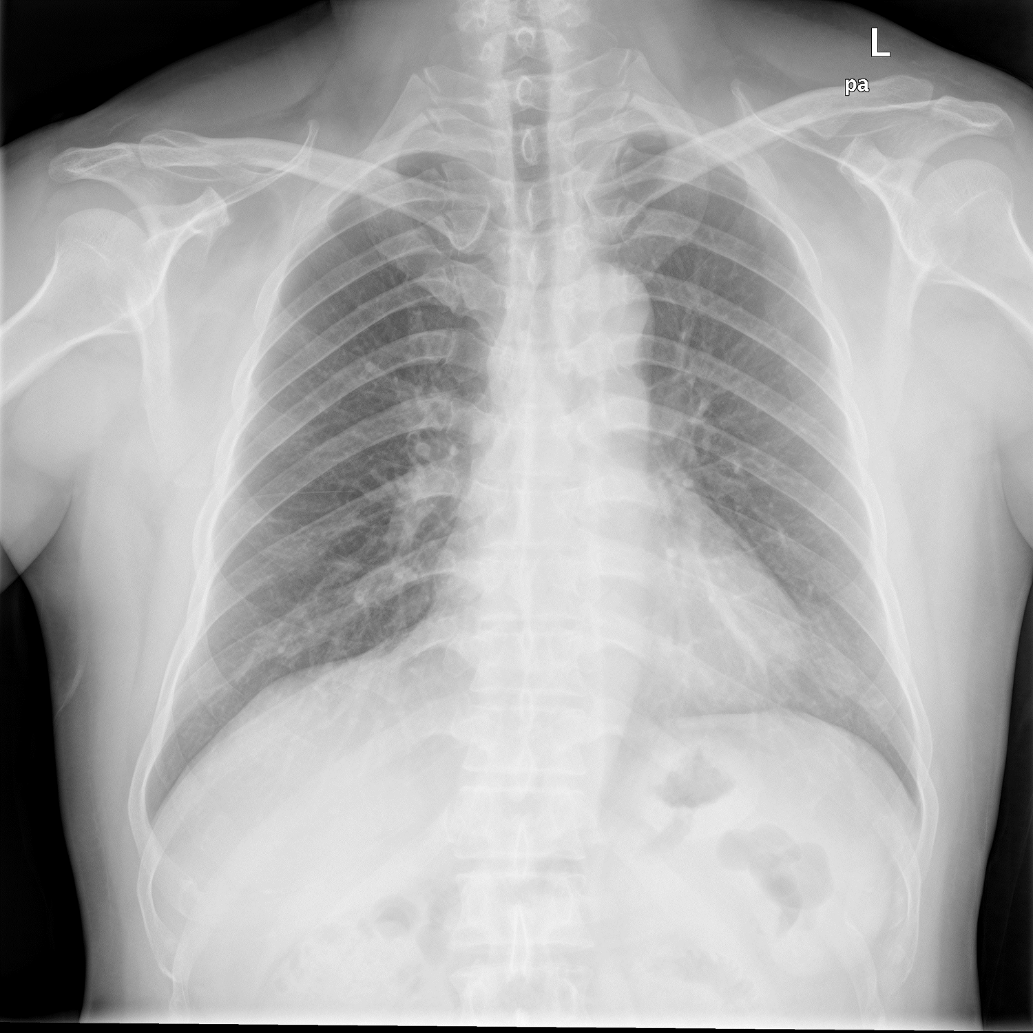
X-Ray – Healthy Lungs
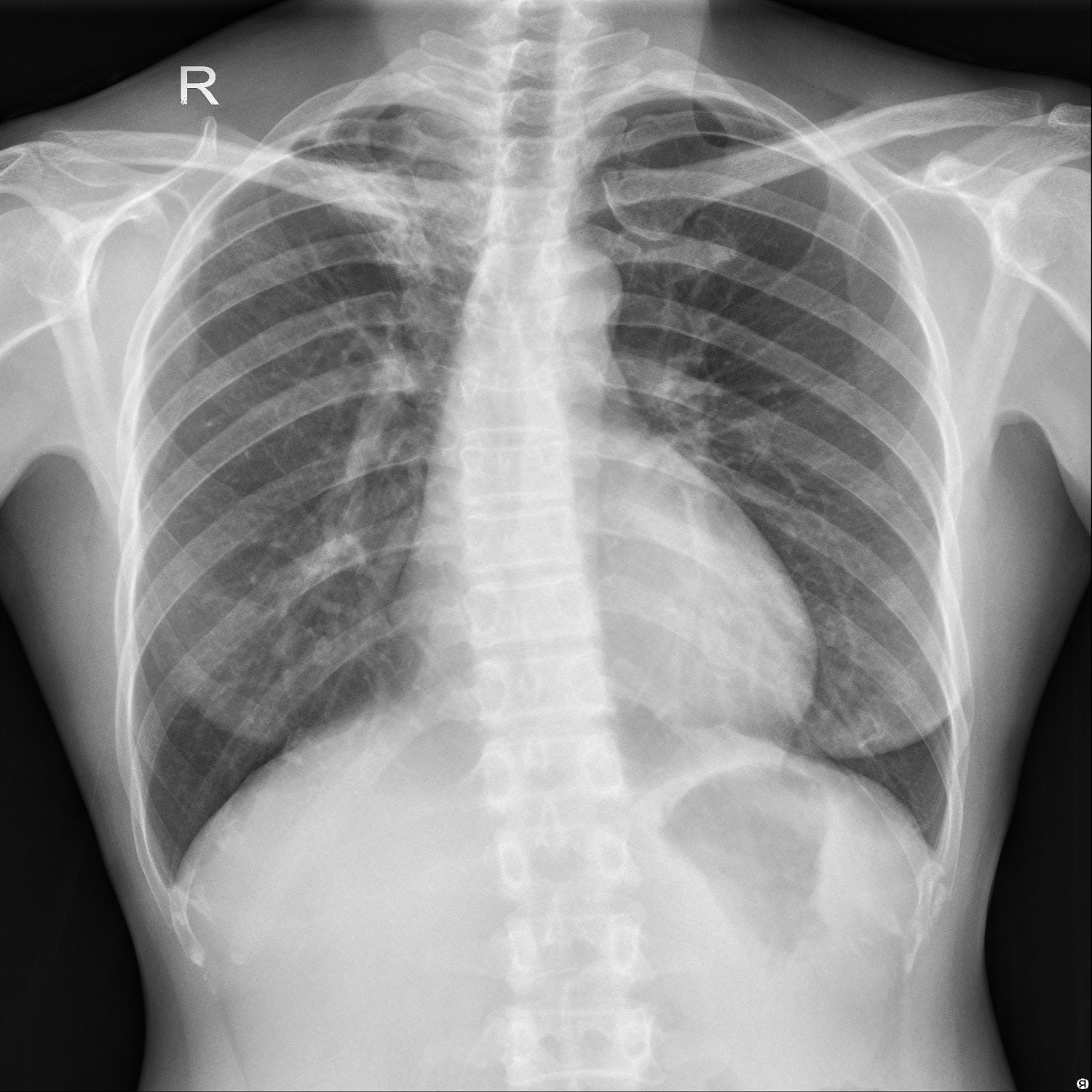
X-Ray – Lungs withTuberculosis
Above Images are sample chest X-Ray images of a normal person and the person having tuberculosis.
file_list=glob.glob("D:/Images/*.png") #Replace the path with the Image folder path
image_list=pd.DataFrame(columns=['path','file_name','label']) #creating a new dataframe to store the image attributes
for i in file_list:
    path=i
    file_name=i.split('\\')[1]
    label=file_name.split('_')[2].replace('.png',"")
    data=path,file_name,label
    image_list=image_list.append({'path':path,'file_name':file_name,'label':label},ignore_index=True)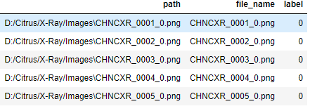
The above code snip will get the all the .png images in the folder and get the filename, file label and file path for all the images and store it into a data frame.
Step 3 - Data Preprocessing and Data split to Training and Testing
Let’s check the distribution of two classes (normal and Tuberculosis)
import matplotlib.pyplot as plt
%matplotlib inline
count = image_list['label'].value_counts(sort = True)
colors = ["grey","orange"]
labels=['Normal','Tuberculosis']
#plotting pie chart
plt.pie(count,labels=labels, colors=colors,autopct='%1.1f%%', shadow=True)
plt.title('Tuberculosis Percentage in data')
plt.show()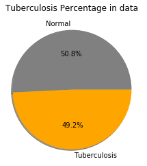
The distribution of labels is almost equal. So, no need to do any data sampling, if we see lesser accuracy after training than we can do data augmentation.
independent=image_list.drop("label",axis=1)
dependent=image_list['label']
X_train, X_test, y_train, y_test = train_test_split(independent, dependent, test_size=0.2, random_state=42)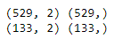
Above step will Split the data into training and testing for further preprocessing
train_image=[]
for index,row in X_train.iterrows():
    img = image.load_img(row[0],target_size=(256,256),color_mode="grayscale") #images are grayscale not color
    img = image.img_to_array(img)
    img = img/255 #standardize the data
    train_image.append(img)
X = np.array(train_image) #converting to NumPy array
X=X.astype('float32')
test_image = []
for index,row in X_test.iterrows():
    #print(row[0],row[1])
    #s3.download_file(bucket,row[0],row[1])
    img = image.load_img(row[0],target_size=(256,256),color_mode="grayscale")
    img = image.img_to_array(img)
    img = img/255
    test_image.append(img)
Test = np.array(test_image)
Test=Test.astype('float32')
The above code will load the image and resize all the images in to 256*256 and store it into list and then convert the list to NumPy array and change the type to float32.
train_label = keras.utils.to_categorical(y_train, 2)
test_labels = keras.utils.to_categorical(y_test, 2)
Convert labels into the format that Keras expects.
Step 4 - Data Preprocessing
We can train the model in two ways; one way is to build the model from the scratch using Keras and other way is to use the existing network architecture and train the model on the top of the network.
First Approach:
Define the network from the scratch
model = Sequential()

model.add(Conv2D(64, (3, 3), padding='same', input_shape=(256, 256, 1), activation="relu"))
model.add(Conv2D(64, (3, 3), activation="relu"))
model.add(MaxPooling2D(pool_size=(2, 2)))
model.add(Dropout(0.25))

model.add(Conv2D(128, (3, 3), padding='same', activation="relu"))
model.add(Conv2D(128, (3, 3), activation="relu"))
model.add(MaxPooling2D(pool_size=(2, 2)))
model.add(Dropout(0.25))

model.add(Conv2D(256, (3, 3), padding='same', activation="relu"))
model.add(Conv2D(256, (3, 3), activation="relu"))
model.add(MaxPooling2D(pool_size=(2, 2)))
model.add(Dropout(0.3))

model.add(Flatten())
model.add(Dense(512, activation="relu"))
model.add(Dropout(0.5))
model.add(Dense(2, activation="sigmoid"))
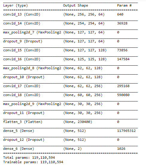
Created a network architecture with 3 hidden layers, each hidden layer is activated with relu function, and the kernel size is (3,3) and added 25% dropout after every hidden layer. The input shape is [256,256,1]. Used sigmoid function in the final layer for the binary classification.
model.summary()
model.compile(
    loss='binary_crossentropy',
    optimizer='adam',
    metrics=['accuracy']
)
The loss function was set to ‘binary_crossentropy’ as we are working on binary classification and optimize used is ‘adam’ and accuracy is chosen as a metric.
model.fit(
    X,
    train_label,
    batch_size=32,
    epochs=30,
    validation_data=(Test, test_labels),
    shuffle=True
)
In the above code we are training the model by passing images randomly in batch size of 32 and checking the accuracy using the test data. We ran this for 30 epochs.
model_structure = model.to_json()
f = Path("model_structure.json")
f.write_text(model_structure) # saving the model architecture
model.save_weights("D:/Citrus/X-Ray/model_weights.h5") # saving the model weights
In the above code snipped we are saving the model network architecture to the json file and saving the model weights. We can use the saved weights to classify the incoming images.
def XRay(name):
    data1=[]
    img = image.load_img(name,target_size=(256,256))
    img = image.img_to_array(img)
    img = img/255
    X = np.array(img)
    X=X.astype('float32')
    Y=X.reshape(1,256,256,3)
    with graph.as_default():
        value = model.predict(Y)
    #print(value)
    if value[0][1]>0.5:
        probability=value[0][1]
        disease = "Patient has Tuberculosis"
        data=probability,disease
        data1.append(data)
    else:
        probability=value[0][1]
        disease = "Patient is Healthy"
        data=probability,disease
        data1.append(data)
    Image_details=pd.DataFrame(data1,columns=['Probability','Disease'])
    Image_details=Image_details.to_json(orient='records')
    return Image_details
Above function will help you to predict the output if you pass the input image.
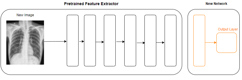
Second Approach (Transfer Learning):
In this approach we will use one of the pretrained neural network architecture which is trained on Imagenet data. VGG16 is a deep neural network with 16 layers, we will use this neural network architecture to extract the features of the incoming image. Below we will discuss how we can use this pretrained model and train our images on the top of this architecture.
images=[]
labels=[]
for index,row in X_train.iterrows():
    # Load the image from drive
    img = image.load_img(row[0],target_size=(256,256))
    # Convert the image to a numpy array
    image_array = image.img_to_array(img)
    # Add the image to the list of images
    images.append(image_array)
    #add corresponding image label
    label=y_train[index]
    labels.append(label)
x_train = np.array(images)
y_train = np.array(labels)
x_train = vgg16.preprocess_input(x_train) #to standardize the data
Above code will load the training images from the drive and resize the image and convert in to NumPy array.
# Load a pre-trained neural network to use as a feature extractor
pretrained_nn = vgg16.VGG16(weights='imagenet', include_top=False, input_shape=(256, 256, 3)) # top=False will remove the output dense layer
features_x = pretrained_nn.predict(x_train) # Extract features for each image (all in one pass)
Here we are loading pre-trained neural network vgg16 to extract the features, we removed the dense layer which maps to the specific output from this pre-trained neural network. Extracted all the training images features.
# Create a model and add layers
model = Sequential()
model.add(Flatten(input_shape=features_x.shape[1:]))
model.add(Dense(256, activation='relu'))
model.add(Dropout(0.5))
model.add(Dense(1, activation='sigmoid'))

# Compile the model
model.compile(
    loss="binary_crossentropy",
    optimizer="adam",
    metrics=['accuracy']
)

# Train the model
model.fit(
    x_train,
    y_train,
    epochs=15,
    shuffle=True
)

# Save neural network structure
model_structure = model.to_json()
f = Path("model_structure.json")
f.write_text(model_structure)

# Save neural network's trained weights
model.save_weights("model_weights.h5")
Above code will create a new neural network model by taking input as extracted features from VGGNet and added a dense layer connected to the output layer. Finally trained the model with training data and save the model architecture and model weights for testing.
Bulk Predictions:
Below code will give the predictions for new images.
# Load the json file that contains the model's structure
from keras.models import model_from_json
f = Path("model_structure.json")
model_structure = f.read_text()

# Recreate the Keras model object from the json data
model = model_from_json(model_structure)

# Re-load the model's trained weights
model.load_weights("model_weights.h5")

#create the array for input test images
test_images=[]
for index,row in X_test.iterrows():
    # Load the image from disk
    img = image.load_img(row[0],target_size=(256,256))

    # Convert the image to a numpy array
    image_array = image.img_to_array(img)

    # Add the image to the list of images
    test_images.append(image_array)

x_test_images = np.array(test_images)
x_test_1 = vgg16.preprocess_input(x_test_images)

# Extracting features from the input images
feature_extraction_model = vgg16.VGG16(weights='imagenet', include_top=False, input_shape=(256, 256, 3))
features = feature_extraction_model.predict(x_test_1)

# Given the extracted features, make a final prediction using our own model
results = model.predict(features)
This is how we will predict the output for the new images. When anyone can use Transfer Learning:
- Always try it first because it is quick and fast.
- Very useful when you don’t have lot of training data but already have a model that solves similar problem
- It will cut the time to train the network from scratch
Conclusion
The impact of using this kind of solutions affect the entire radiology value chain as the tasks gets automated that results in the elimination of the Processes. AI solution in healthcare can improve efficiency by lowering down the costs and saving time. Using AI, BigData sets can be analyzed and doctors can leverage a 360-degree vision of their patient health history resulting in better care of the patient.
Artificial Intelligence can improve the diagnostics quality by reducing human errors, accurately analyzing large amount of data, quantifying reports and integrating data. Key areas of the patient health ecosystem can be discovered with the help of Artificial Intelligence.
On the closing note, I would like to emphasize the fact that AI algorithms should be taken as additional support for making important decisions specially in domains such as healthcare.


